Oblique Shock
Repository path: tutorials/singleRegion/rhoPimpleFluid/obliqueShock
Tutorial aims
- Demonstrate how to run
rhoPimpleFluidin single-region mode on a compressible, supersonic problem with a standing shock. - Demonstrate local time stepping (LTS, the
localEulerddtscheme) as a pseudo-transient path to a steady-state solution. - Demonstrate a
transonic yesPIMPLE setup and the associated pressure-limiting controls (pMin/pMax). - Validate the region type’s predicted pressure, temperature and velocity jump across an oblique shock against classical θ-β-M shock theory.
Case Overview
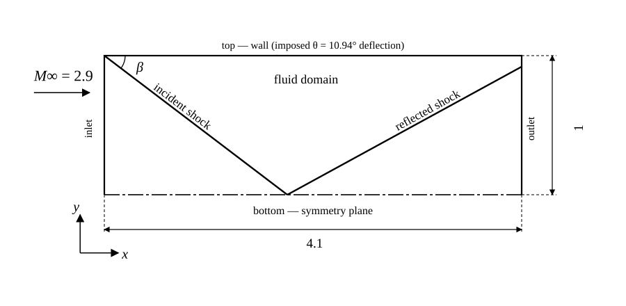
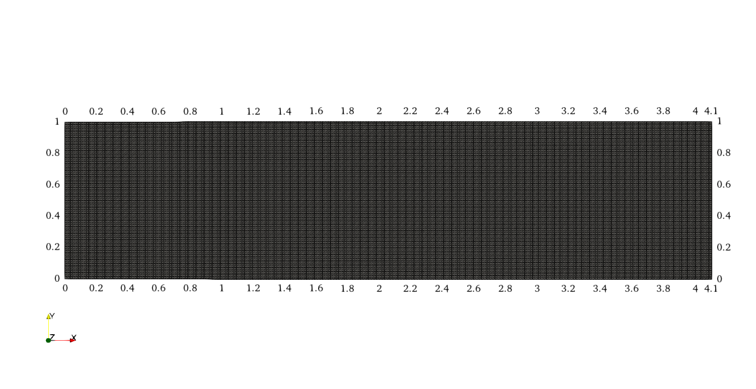 Case geometry and mesh: a 4.1 × 1 rectangular domain, 240 × 120 cells, with the wedge deflection imposed as a boundary condition on the
top patch rather than meshed as a physical wedge.
This case computes the steady oblique shock produced when a Mach 2.9 supersonic stream is deflected by 10.94°. It is the multiPhysicsFoam counterpart of the stock OpenFOAM rhoCentralFoam obliqueShock tutorial: the same domain, mesh topology and boundary values are reused, but the problem is solved through the multiPhysicsFoam framework using the rhoPimpleFluid region type running in single-region mode, marched to steady state with local time stepping instead of rhoCentralFoam’s explicit density-based time integration.
Rather than meshing a physical wedge, the deflection is imposed directly as a boundary condition: the top patch (declared type wall in blockMeshDict) carries fixedValue conditions on U and T corresponding to the post-deflection state, while p on top is left zeroGradient — the post-shock pressure is therefore a genuine prediction of the solver, not an imposed value, which is what makes this case a validation case rather than a demonstration.
| Patch | Type | Role |
|---|---|---|
inlet | patch | Supersonic inflow, $M = 2.9$ |
top | wall | Imposed deflected-flow wall (fixedValue U, T; zeroGradient p) — represents the wedge |
bottom | symmetryPlane | Flow symmetry axis; the incident shock reflects here |
outlet | patch | zeroGradient outflow |
frontAndBack | empty | 2D case (one cell thick) |
The gas is a normalised perfect gas (molWeight 11640.3, Cp 2.5, mu 0), chosen so that at T = 1 the speed of sound is $c \approx 1$ — the inlet condition U = (2.9\ 0\ 0) is therefore Mach 2.9 by construction, and any velocity magnitude in the case can be read directly as a Mach number.
The governing equations solved by rhoPimpleFluid are the compressible continuity, momentum and enthalpy-energy equations (see regions/rhoPimpleFluid.md for the full derivation):
Since mu 0 and simulationType laminar, both the effective stress $\mathbf{R}$ and the effective thermal diffusivity $\alpha_\text{eff}$ vanish identically — the momentum and energy equations reduce to their inviscid (Euler) form, and the shock is captured purely by the convection schemes (vanLeerV, limitedLinear), not by physical diffusion.
For a weak oblique shock, the wave angle $\beta$, upstream Mach number $M_1$ and flow-deflection angle $\theta$ are related by the θ-β-M relation:
$$ \tan\theta = \frac{2\cot\beta\left(M_1^2\sin^2\beta - 1\right)}{M_1^2\left(\gamma + \cos 2\beta\right) + 2} $$with the pressure ratio across the shock given by
$$ \frac{p_2}{p_1} = 1 + \frac{2\gamma}{\gamma+1}\left(M_1^2\sin^2\beta - 1\right) $$At $M_1 = 2.9$ and $\theta = 10.94°$ (the deflection imposed on top), the weak-shock solution is $\beta = 29.0°$ exactly — substituting $\beta = 29°$ back into the relation above reproduces $\tan\theta = 0.1933$, the same ratio as the imposed velocity components on top (2.61933/0.50632), confirming the case was designed backwards from $\beta = 29°$. This is the analytic target the Results section below validates against.
Case Structure
The case structure follows the typical OpenFOAM case structure:
obliqueShock
├── 0.orig
│   ├── p
│   ├── T
│   └── U
├── Allclean
├── Allrun
├── constant
│   ├── thermophysicalProperties
│   └── turbulenceProperties
└── system
    ├── blockMeshDict
    ├── controlDict
    ├── fvSchemes
    └── fvSolution
0.orig— initial and boundary conditions for the primitive fieldsp,T,U.constant/thermophysicalProperties— the equation of state, transport model and energy variable.constant/turbulenceProperties— the turbulence model selection (laminarhere).system/blockMeshDict— the block-structured mesh (240×120 cells, generated at run time).system— the run-time control (controlDict), discretization schemes (fvSchemes) and linear-solver/PIMPLE settings (fvSolution).
The key entries that select the physics are in system/controlDict:
application       multiPhysicsFoam;

singleRegionMode yes;

regionType       rhoPimpleFluid;
application multiPhysicsFoam: the executable that is run.singleRegionMode yes: tells the framework there is only one region occupying the whole domain, so noconstant/regionProperties/multi-region setup is required.regionType rhoPimpleFluid: selects therhoPimpleFluidregion type at runtime.
Initial Conditions and Boundary Conditions
There are three primitive variables:
├── 0.orig
│   ├── p   pressure scalar field
│   ├── T   temperature scalar field
│   └── U   velocity vector field
Pressure Field p
dimensions      [1 -1 -2 0 0 0 0];

internalField   uniform 1;

boundaryField
{
    top
    {
        type            zeroGradient;
    }

    inlet
    {
        type            fixedValue;
        value           uniform 1;
    }

    outlet
    {
        type            zeroGradient;
    }

    bottom
    {
        type            symmetryPlane;
    }

    frontAndBack
    {
        type            empty;
    }
}
topiszeroGradient— deliberately unconstrained, so the post-shock pressure is a solver prediction.inletis held at the free-stream pressure,1.outletiszeroGradient, a standard supersonic outflow condition.bottomis asymmetryPlane, reflecting the incident shock.
Temperature Field T
dimensions      [0 0 0 1 0 0 0];

internalField   uniform 1;

boundaryField
{
    top
    {
        type            fixedValue;
        value           uniform 1.25853;
    }

    inlet
    {
        type            fixedValue;
        value           uniform 1;
    }

    outlet
    {
        type            zeroGradient;
    }

    bottom
    {
        type            symmetryPlane;
    }

    frontAndBack
    {
        type            empty;
    }
}
topis fixed at1.25853— the analytic post-shock temperature ratio $T_2/T_1 = 1.2585$ from the θ-β-M solution, matching to 4 significant figures.inletis held at the free-stream temperature,1.
Velocity Field U
dimensions      [0 1 -1 0 0 0 0];

internalField   uniform (2.9 0 0);

boundaryField
{
    top
    {
        type            fixedValue;
        value           uniform (2.61933 -0.50632 0);
    }

    inlet
    {
        type            fixedValue;
        value           uniform (2.9 0 0);
    }

    outlet
    {
        type            zeroGradient;
    }

    bottom
    {
        type            symmetryPlane;
    }

    frontAndBack
    {
        type            empty;
    }
}
topis fixed at(2.61933 -0.50632 0)— the exact post-deflection velocity, with the ratio of its components ($\arctan(0.50632/2.61933) = 10.94°$) fixing the imposed deflection angle $\theta$.inletis held at Mach 2.9,(2.9 0 0).
Thermophysical Properties
thermoType
{
    type            hePsiThermo;
    mixture         pureMixture;
    transport       const;
    thermo          hConst;
    equationOfState perfectGas;
    specie          specie;
    energy          sensibleEnthalpy;
}

mixture
{
    // normalised gas
    specie
    {
        molWeight       11640.3;
    }
    thermodynamics
    {
        Cp              2.5;
        Hf              0;
    }
    transport
    {
        mu              0;
        Pr              1;
    }
}
The gas constant follows from molWeight: $R = 8314.47/11640.3 = 0.71411$, so $C_v = C_p - R = 1.78589$ and $\gamma = C_p/C_v = 1.39985$. At T = 1 the speed of sound is $c = \sqrt{\gamma R T} = 0.99988 \approx 1$, which is why the inlet velocity 2.9 reads directly as $M_1 = 2.9$. mu 0 makes the fluid inviscid.
Turbulence Properties
simulationType laminar;
Note
There is no momentumTransport file in this case — rhoPimpleFluid reads turbulenceProperties. Combined with mu 0 above, the case has no molecular or turbulent diffusion at all: momentum and energy transport are purely convective, so the shock is resolved entirely by the shock-capturing convection schemes in fvSchemes.
Numerical Setup
system/fvSchemes:
ddtSchemes  { default localEuler; }

gradSchemes
{
    default  cellLimited Gauss linear 1;
    grad(p)  cellLimited Gauss linear 0.333;
    grad(h)  cellLimited Gauss linear 0.333;
}

divSchemes
{
    default         none;
    div(phi,U)      Gauss vanLeerV;
    div(phi,K)      Gauss linear;
    div(phi,h)      Gauss limitedLinear 1;
    div(phid,p)     Gauss limitedLinear 1;
    div(phiv,p)     Gauss limitedLinear 1;
    div(((rho*nuEff)*dev2(T(grad(U))))) Gauss linear;
}

laplacianSchemes     { default Gauss linear limited 1; }
interpolationSchemes { default linear; }
snGradSchemes        { default limited 1; }
ddtSchemes { default localEuler; } selects local time stepping: each cell marches at its own locally-limited pseudo-time step towards steady state, rather than the whole domain sharing one physical time step. div(phi,U) Gauss vanLeerV and the limitedLinear entries are TVD/limited schemes chosen to capture the shock without spurious oscillations. The div(((rho*nuEff)*dev2(T(grad(U))))) entry is the viscous-stress divergence term; it is present for completeness but numerically inert here since nuEff = mu/rho = 0.
system/fvSolution:
solvers
{
    p
    {
        solver PBiCGStab;
        preconditioner DILU;
        tolerance 1e-06;
        relTol 0.01;
        minIter 2;
    }

    pFinal
    {
        $p;
        relTol 0;
        minIter 2;
    }

    "(U.*|h.*)"
    {
        solver PBiCGStab;
        preconditioner DILU;
        tolerance 1e-08;
        relTol 0;
        minIter 2;
    }

    "rho.*"
    {
        solver diagonal;
    }
}

PIMPLE
{
    momentumPredictor        yes;
    nOuterCorrectors         1;
    nCorrectors              3;
    nNonOrthogonalCorrectors 2;
    transonic                yes;
    maxCo                    0.5;
    rDeltaTSmoothingCoeff    0.1;
    rDeltaTDampingCoeff      0.9;
    maxDeltaT                1;
    pMin                     0.1;
    pMax                     10;
}

relaxationFactors
{
    equations
    {
        ".*" 1;
    }
}
nOuterCorrectors 1 means there is no outer PIMPLE loop — the solver runs in plain PISO mode, confirmed by the solver’s own start-up message PIMPLE: Operating solver in PISO mode. transonic yes adds the acoustic (phid-based) Courant contribution needed for a flow that spans subsonic and supersonic regions. maxCo, rDeltaTSmoothingCoeff, rDeltaTDampingCoeff and maxDeltaT are LTS controls: the region reads them each iteration to recompute its per-cell reciprocal pseudo-time step rDeltaT, smoothing and damping its rate of change so the pseudo-time march stays stable near the shock. pMin/pMax bound the pressure field via pressureControl, guarding the iterative march (which starts far from the converged state) against unphysical pressures.
Note
With ddtSchemes { default localEuler; } and controlDict’s adjustTimeStep no, deltaT 1, endTime 1000, the solver’s “Time” axis is really a pseudo-iteration counter — 1000 LTS iterations to steady state — not a physical time coordinate. The top-level maxCo 0.5/maxDeltaT 1 entries in controlDict are inert under LTS; the controls that matter are the ones inside the PIMPLE sub-dict above.
Running the Case
As in all multiPhysicsFoam tutorials, the case is run using the included Allrun script, i.e. > ./Allrun. In this case, the Allrun script is:
#!/bin/sh
cd "${0%/*}" || exit                                # Run from this directory
. ${WM_PROJECT_DIR:?}/bin/tools/RunFunctions        # Tutorial run functions
#------------------------------------------------------------------------------


restore0Dir

runApplication blockMesh

runApplication $(getApplication)

#------------------------------------------------------------------------------
The script restores the initial 0 directory from 0.orig, meshes the domain with blockMesh, then reads the application entry from system/controlDict (here multiPhysicsFoam) via $(getApplication) and runs it.
Examining the Solver Output
At start-up, the framework reports the region it has created, the PIMPLE mode, the thermodynamics package and the LTS/pressure-limiting controls:
Creating multi-region system

Creating regions:
Creating region region0: rhoPimpleFluid
Selecting regionType: rhoPimpleFluid

PIMPLE: Operating solver in PISO mode

Selecting thermodynamics package
{
    type            hePsiThermo;
    mixture         pureMixture;
    transport       const;
    thermo          hConst;
    equationOfState perfectGas;
    specie          specie;
    energy          sensibleEnthalpy;
}

No MRF models present

Using LTS
pressureControl
    pMax 10
    pMin 0.1

Selecting turbulence model type laminar
Selecting laminar stress model Stokes

Creating region interfaces:
Since this is a single-region case, no region interfaces are created. Each pseudo-iteration then reports the flow time scale, the PIMPLE predictor/corrector stages, and the linear-solver residuals:
Time = 1
Time step = 1 Index = 1

Flow time scale min/max = 0.00257872, 0.0029454
Smoothed flow time scale min/max = 0.00257872, 0.0029454
Solved region specific physics in 0 s.
Pre-predictor for rhoPimpleFluid in region region0
Momentum predictor for rhoPimpleFluid in region region0
diagonal:  Solving for rho, Initial residual = 0, Final residual = 0, No Iterations 0
DILUPBiCGStab:  Solving for Ux, Initial residual = 1, Final residual = 1.67672e-64, No Iterations 2
DILUPBiCGStab:  Solving for Uy, Initial residual = 1, Final residual = 3.17512e-64, No Iterations 2
DILUPBiCGStab:  Solving for h, Initial residual = 1, Final residual = 7.11843e-65, No Iterations 2
Pressure corrector for rhoPimpleFluid in region region0
DILUPBiCGStab:  Solving for p, Initial residual = 1, Final residual = 1.50964e-06, No Iterations 2
DILUPBiCGStab:  Solving for p, Initial residual = 0.0504941, Final residual = 7.35055e-08, No Iterations 2
DILUPBiCGStab:  Solving for p, Initial residual = 0.00893649, Final residual = 1.30098e-08, No Iterations 2
diagonal:  Solving for rho, Initial residual = 0, Final residual = 0, No Iterations 0
time step continuity errors : sum local = 8.21581e-06, global = 8.21574e-06, cumulative = 8.21574e-06
Solved PIMPLE without coupling in 0.27 s.
ExecutionTime = 0.69 s  ClockTime = 1 s
The important lines are:
PIMPLE: Operating solver in PISO mode: reports thatnOuterCorrectors 1, i.e. no outer loop.Using LTS: confirms thelocalEulerscheme is active and the region is maintaining its ownrDeltaTfield.Pre-predictor/Momentum predictor/Pressure corrector for rhoPimpleFluid in region region0: the three PIMPLE hooks (prePredictor,momentumPredictor,pressureCorrector), driven once per iteration byregionTypeList::solvePIMPLE()sinceusesPIMPLE()istruefor this region.DILUPBiCGStab: Solving for …, Initial residual = …, Final residual = …: the linear-solver report for each field, per the solver settings infvSolution.Solved PIMPLE without coupling in … s.: confirms the region has been solved with no partitioned inter-region (DNA) coupling, since this is a single-region case.
Rather than decaying monotonically to machine precision, the initial residual for p drops rapidly over the first ~100 iterations from 1 to about 0.004, then plateaus in the 0.002–0.004 range for the remainder of the run — expected behaviour for a steady problem with a standing shock, where the sharp discontinuity keeps a small but persistent residual alive at the shock front:
Time=1    Initial residual = 1
Time=2    Initial residual = 0.278001
Time=5    Initial residual = 0.0767708
Time=10   Initial residual = 0.0339211
Time=20   Initial residual = 0.0157623
Time=50   Initial residual = 0.00661829
Time=100  Initial residual = 0.00381484
Time=200  Initial residual = 0.00280615
Time=300  Initial residual = 0.0033075
Time=400  Initial residual = 0.00363008
Time=500  Initial residual = 0.00212176
The run reaches the configured endTime and exits cleanly:
Solved PIMPLE without coupling in 0.15 s.
ExecutionTime = 196.96 s  ClockTime = 198 s

End
Results (validation)
The case was run to endTime 1000 and the converged fields sampled along a horizontal line at $y = 0.5$ (mid-height, ahead of where the reflected shock arrives) and, for the pressure jump, by area-averaging over the top patch:
| Quantity | Analytic ($\beta = 29.0°$) | Measured (this run) | Where measured |
|---|---|---|---|
| Wave angle $\beta$ | $29.0°$ | crosses $y=0.5$ between $x \approx 0.83$–$0.99$ (predicted $0.90$); crosses bottom between $x \approx 1.78$–$1.86$ (predicted $1.804$) | pressure-jump location along sampled lines |
| $p_2/p_1$ | $2.1394$ | $2.1398$ (mid-height plateau mean, $1.1 \le x \le 2.9$) | postProcess -func sampled line, field p |
| $T_2/T_1$ | $1.2585$ | $1.2592$ | same sampled line, field T |
| $U_2$ (m/s) | $(2.61933,\ -0.50632)$ | $(2.6185,\ -0.5061)$ | same sampled line, field U |
| $M_2$ | $2.378$ | $2.377$ (computed from measured $T_2$, $U_2$) | derived from the row above |
$p$, area-averaged on top | $2.1394$ | $2.1334$ | postProcess -func "patchAverage(name=top, p)" |
All measured quantities agree with the analytic θ-β-M solution to within 0.1%. The top-patch area average is slightly lower than the mid-height plateau value because it also includes a small corner region near inlet that lies ahead of the shock at $p = 1$; the mid-height plateau (sampled between the incident shock and before the reflected shock arrives) is the cleaner comparison.
Sampling further downstream (past $x \approx 3.0$) shows a second pressure rise, to $p \approx 4.0$–$4.3$ — the incident shock reflecting off the bottom symmetry plane and compressing the flow a second time. This is expected shock-reflection physics, not a discrepancy: the single-shock analytic values above only apply in the region between the incident shock and the reflection.
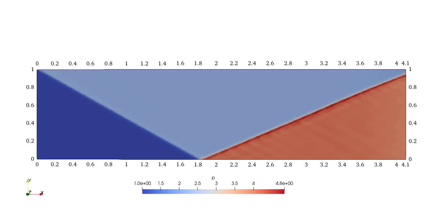 Pressure field at the final iteration, showing the incident shock at β ≈ 29° emanating from the top-left corner and reflecting off the
bottom symmetry plane.
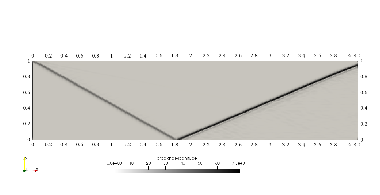 Recreation of a numerical Schlieren image of the incident and reflected shocks, using Paraview’s gradient filter applied to density.