Pitz Daily
Repository path: tutorials/singleRegion/potentialFluid/pitzDaily
Tutorial aims
- Demonstrate how to solve an inviscid, irrotational potential-flow problem using the
potentialFluidregion type. - Demonstrate how to perform a single-region analysis in multiPhysicsFoam.
- Demonstrate the use of
potentialFluidas an initialiser that generates a divergence-free starting field for a subsequent Navier-Stokes run. - Illustrate, by construction, the physical limits of the potential-flow model.
Case Overview
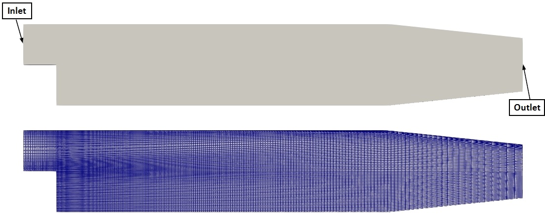 Case geometry and mesh
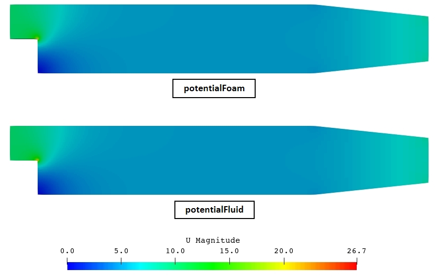
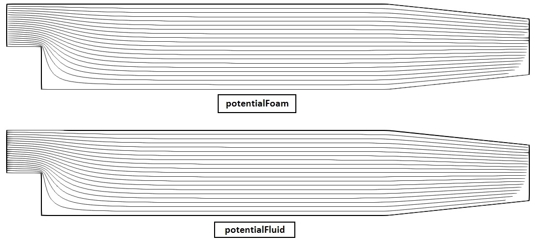
This case computes the two-dimensional potential flow through the Pitz-Daily backward-facing step geometry. It is the multiPhysicsFoam counterpart of the OpenFOAM potentialFoam pitzDaily tutorial: the same geometry, mesh and boundary conditions are used, but the problem is solved through the multiPhysicsFoam framework using the potentialFluid region type running in single-region mode.
The geometry is a sudden expansion followed by a contracting nozzle, meshed with 12225 hexahedral cells one cell thick in $z$ (the blockMeshDict is specified in millimetres and scaled by 0.001). A uniform velocity of 10 m/s enters at the inlet upstream of the step.
The same mesh is used by the pimpleFluid pitzDaily tutorial, which makes this case a natural demonstration of the initialiser workflow: the potential-flow field computed here is a valid, discretely divergence-free starting point for a full turbulent Navier-Stokes solve on the same grid.
The governing model assumes the fluid is incompressible and irrotational:
$$ \nabla \cdot \mathbf{U} = 0 \qquad\qquad \nabla \times \mathbf{U} = 0 $$Irrotationality permits the velocity to be written as the gradient of a scalar velocity potential $\Phi$, and substituting into continuity reduces the whole problem to a single Laplace equation:
$$ \mathbf{U} = \nabla \Phi \qquad \Longrightarrow \qquad \nabla^2 \Phi = 0 $$There is no viscosity, no time derivative and no pressure-velocity coupling - the flow is determined entirely by the boundary conditions.
In practice potentialFluid does not solve $\nabla^2 \Phi = 0$ literally. It starts from the face-flux field $\phi^{*}$ implied by the boundary conditions alone and removes its divergent part, which is equivalent but guarantees discrete continuity on the actual mesh:
so that $\nabla \cdot \phi = 0$ to solver tolerance. The cell-centred velocity is then recovered from the corrected fluxes:
for all time-steps
    make phi relative to MRF zones
    adjustPhi: balance global in/outflow if pKin needs a reference
    for nNonOrthogonalCorrectors + 1 iterations
        construct PhiEqn:  laplacian(Phi) == div(phi)
        setReference(PhiRefCell, PhiRefValue)
        solve PhiEqn for Phi
        if final non-orthogonal iteration:
            phi -= PhiEqn.flux()
    make phi absolute
    report continuity error
    U = reconstruct(phi);  U.correctBoundaryConditions()
    report interpolated velocity error
    if writep:
        construct and solve pKinEqn:  laplacian(pKin) + div(F & div(phi,U)) == 0
    update dimensional pressure p = pKin*rho
end
Warning
This case does not model the real physics of a backward-facing step. The defining feature of the Pitz-Daily flow is the recirculation zone behind the step, which is produced by viscous separation. Potential flow has no viscosity, so the computed solution turns the corner cleanly with no separation, no recirculation and no wake. That is not a defect in the case - it is what the model says. The case is included as a smoke test and as an initialiser demonstration, and it is a useful illustration of exactly what potential flow leaves out.
Note
potentialFoam has no time loop at all - it solves once and exits. multiPhysicsFoam has a real time loop, and solveRegion() is therefore called on every time step. The solve is deliberately not latched, so this case restricts the run to a single step through controlDict (endTime 1; deltaT 1;). This reproduces potentialFoam’s one-shot behaviour exactly.
Case Structure
The case structure follows the typical OpenFOAM case structure:
pitzDaily
├── 0.orig
│   ├── U
│   └── pKin
├── Allclean
├── Allrun
├── constant
│   ├── polyMesh
│   │   └── …
│   └── transportProperties
└── system
    ├── blockMeshDict
    ├── controlDict
    ├── fvSchemes
    └── fvSolution
0.orig- initial and boundary conditions, copied to0byrestore0Dirat the start ofAllrun.constant/transportProperties- the fluid densityrho.constant/polyMesh- the mesh (generated at run time byblockMesh).system- the run-time control (controlDict), the mesh definition (blockMeshDict), discretization schemes (fvSchemes) and linear-solver and region settings (fvSolution).
The single write time produces:
1
├── Phi              velocity potential
├── U                velocity
├── p                dimensional pressure
├── pKin             kinematic pressure
├── phi              volumetric face flux
├── streamFunction   (postProcess)
└── uniform
The key entries that select the physics are in system/controlDict:
application       multiPhysicsFoam;

singleRegionMode yes;

regionType       potentialFluid;
application multiPhysicsFoam: the executable that is run.singleRegionMode yes: tells the framework there is only one region occupying the whole domain, so noconstant/multiRegionProperties/multi-region setup is required.regionType potentialFluid: selects thepotentialFluidregion type at runtime.
The time controls limit the run to exactly one step:
endTime          1;
deltaT           1;
writeControl     timeStep;
writeInterval    1;
adjustTimeStep   no;
Note
adjustTimeStep no is belt-and-braces. potentialFluid::getMinDeltaT() returns GREAT, which the framework’s setDeltaT.H already interprets as “this region imposes no time-step constraint”, so the step size would not be modified even with adjustment enabled.
Initial Conditions and Boundary Conditions
In this case, there are two supplied fields:
├── 0.orig
│   ├── U      velocity vector field
│   └── pKin   kinematic pressure scalar field
Velocity Field U
dimensions      [0 1 -1 0 0 0 0];

internalField   uniform (0 0 0);

boundaryField
{
    inlet
    {
        type            fixedValue;
        value           uniform (10 0 0);
    }

    outlet
    {
        type            zeroGradient;
    }

    upperWall
    {
        type            noSlip;
    }

    lowerWall
    {
        type            noSlip;
    }

    frontAndBack
    {
        type            empty;
    }
}
inletholds a uniform 10 m/s in $+x$.outletuseszeroGradientso the velocity is free to develop.upperWallandlowerWallarenoSlip.frontAndBackisemptyfor a 2D case.
Note
noSlip on the walls may look inconsistent with an inviscid model, and in a sense it is - but it produces the correct behaviour here. noSlip is a fixedValue condition, so the boundary-condition inference chain makes pKin zeroGradient on those patches and Phi zeroGradient in turn, which enforces zero flux through the wall. Since the velocity is reconstructed from the corrected fluxes rather than taken from the supplied field, the walls behave as impermeable slip walls, which is exactly the potential-flow wall condition. The cylinder tutorial expresses the same intent more directly using symmetry.
Note
potentialFluid zeroes U’s internal field in its constructor, so the internalField uniform (0 0 0) entry above is not really an initial condition - only the boundary conditions of U matter. The potential-flow solution is fully determined by them, so any interior guess is discarded. Note that the constructor also assigns zero to the boundary field, but fixedValueFvPatchField::operator= is a no-op, so the prescribed inlet value survives.
Kinematic Pressure Field pKin
dimensions      [0 2 -2 0 0 0 0];

internalField   uniform 0;

boundaryField
{
    inlet
    {
        type            zeroGradient;
    }

    outlet
    {
        type            fixedValue;
        value           uniform 0;
    }

    upperWall
    {
        type            zeroGradient;
    }

    lowerWall
    {
        type            zeroGradient;
    }

    frontAndBack
    {
        type            empty;
    }
}
Note that pKin is the mirror image of U: wherever U fixes a value (inlet, the walls), pKin is zeroGradient; wherever U is free (outlet), pKin is fixedValue. This is physically necessary - you cannot independently impose both velocity and pressure at the same boundary.
The dimensions [0 2 -2 0 0 0 0] (m²/s²) indicate that pKin is a kinematic pressure, i.e. $p/\rho$.
Note
In potentialFoam this field is simply called p. The port renames it to pKin to follow the multiPhysicsFoam convention (as in pimpleFluid), reserving the name p for the dimensional pressure. One consequence: setRefCell derives its dictionary keywords from the field name, so this case would use pKinRefCell/pKinRefValue, not pRefCell/pRefValue. Neither is needed here, because the fixed-value outlet already anchors the pressure.
Supplying 0/pKin is in fact optional. If it is absent, potentialFluid constructs it with boundary types inferred from U by exactly the inversion described above, and then infers Phi’s boundary types from pKin by inverting again. Supplying 0/U alone is sufficient.
Transport Properties
The only physical property required is the density rho, specified in constant/transportProperties:
rho 1000;
rho is read as a dimensionedScalar with dimDensity, so the bare number above is interpreted as kg/m³ (dimensions are supplied in code).
Note
Density plays no part in the potential-flow solution, which is purely kinematic. It is used only to form the dimensional pressure field (p = pKin * rho) that sibling regions expect. constant/transportProperties is nevertheless mandatory - it is read MUST_READ, and the region will abort without it. This is a difference from stock potentialFoam, whose tutorials contain no transportProperties file at all.
Region Controls - the potentialFlow subdict
system/fvSolution carries the linear solvers and the region-specific controls:
solvers
{
    Phi
    {
        solver          GAMG;
        smoother        DIC;
        tolerance       1e-06;
        relTol          0.01;
    }

    pKin
    {
        $Phi;
    }
}

potentialFlow
{
    nNonOrthogonalCorrectors 2;

    writePhi        true;
    writep          true;
}
potentialFoam is a standalone executable and exposes its options as command-line flags. A region type cannot take command-line arguments, so these become optional entries in the potentialFlow subdict, all read as Foam::Switch and defaulting to false:
| Entry | Upstream flag | Effect |
|---|---|---|
initialiseUBCs | -initialiseUBCs | Call U.correctBoundaryConditions() and rebuild phi before solving. Needed when a boundary condition computes its value from other fields. |
writePhi | -writePhi | AUTO_WRITE the velocity potential Phi |
writep | -writep | Calculate the approximate Euler pressure |
Being Switch-valued, each accepts true/false, yes/no or on/off.
Note
writep gates the calculation, not the writing. U, phi, pKin and p are all AUTO_WRITE unconditionally, because they are primary fields shared with sibling regions on the same mesh and must be writable whichever region owns them. A consequence worth knowing: with writep false, pKin and p are still written, but as zero, because the Euler pressure was never computed. The upstream -writephi flag has no equivalent at all - phi is always written.
nNonOrthogonalCorrectors 2 means the $\Phi$ equation is assembled and solved three times. The implicit Laplacian only captures the face-normal part of the gradient; on a non-orthogonal mesh the remainder is added explicitly and therefore lags, so the equation is re-solved until it settles. The flux correction phi -= PhiEqn.flux() is applied only on the final iteration. This mesh is graded and moderately non-orthogonal, which is why correctors are needed at all.
Running the Case
As in all multiPhysicsFoam tutorials, the case is run using the included Allrun script, i.e. > ./Allrun. In this case, the Allrun script is:
#!/bin/sh
cd "${0%/*}" || exit                                # Run from this directory
. ${WM_PROJECT_DIR:?}/bin/tools/RunFunctions        # Tutorial run functions
#------------------------------------------------------------------------------

restore0Dir

runApplication blockMesh

runApplication $(getApplication)

runApplication postProcess -func streamFunction -latestTime

#------------------------------------------------------------------------------
The script restores the initial 0 directory, generates the mesh with blockMesh, and runs the solver. The $(getApplication) call reads the application entry from system/controlDict (here multiPhysicsFoam) and runs it. Finally postProcess computes the stream function from the solved flux field, which is convenient for visualising streamlines.
Note
The upstream potentialFoam version of this script passes options on the command line: potentialFoam -writePhi -writephi -writep. All of these are gone here - the write/calculate switches moved into the potentialFlow dict.
Note
-latestTime is passed to postProcess deliberately. Without it, postProcess also visits time 0, which contains only U and pKin and no phi, and reports a spurious Field phi not found / failed to execute warning before succeeding at time 1. This is an artefact of the framework advancing time (0 → 1) where potentialFoam wrote everything into 0.
Note
This case is run through the multiPhysicsFoam solver, not potentialFoam.
The choice of physics is made entirely through the case dictionaries - in particular regionType potentialFluid in system/controlDict - so the same executable is used for every multiPhysicsFoam tutorial.
Unlike the cylinder case, this one needs no canCompile guard - there is no dynamic code in either the mesh definition or the function objects.
Examining the Solver Output
Let us examine the output from the multiPhysicsFoam solver for this case.
At start-up, the framework reports the region it has created and the coupling mode:
Creating multi-region system

Creating regions:
Creating region region0: potentialFluid
Selecting regionType: potentialFluid

potentialFlow: Operating solver in PISO mode

No MRF models present

No PIMPLE active

Creating region interfaces:
potentialFlow: Operating solver in PISO mode:potentialFluidconstructs apisoControlnamedpotentialFlow, exactly aspotentialFoamdoes. It is used only for its non-orthogonal corrector loop and its dictionary access - no PISO pressure-velocity iteration takes place.No MRF models present: noconstant/MRFPropertieswas supplied.No PIMPLE active:potentialFluid::usesPIMPLE()returnsfalse, so the framework skips the PIMPLE stage entirely.
Since this is a single-region case, no region interfaces are created. The single time step then reports the potential-flow solution:
Time = 1
Time step = 1 Index = 1


Calculating potential flow in region region0
GAMG:  Solving for Phi, Initial residual = 1, Final residual = 0.00961922, No Iterations 14
GAMG:  Solving for Phi, Initial residual = 0.0117848, Final residual = 6.83576e-05, No Iterations 5
GAMG:  Solving for Phi, Initial residual = 0.000243718, Final residual = 1.35614e-06, No Iterations 9
Continuity error = 0.00269801
Interpolated velocity error = 0.000114117
The important lines are:
Calculating potential flow in region region0: the region announces its solve. The region name isregion0, the default single-region mesh name.- Three
GAMG: Solving for Phireports - one per non-orthogonal corrector iteration (nNonOrthogonalCorrectors 2plus the initial solve). The initial residual falls from1to2.4e-04across the loop, showing the explicit non-orthogonal contribution converging. Continuity error = 2.70e-03: the volume-weighted average of $|\nabla \cdot \phi|$ after the flux correction. This is the primary measure of whether the projection succeeded. It is roughly twenty times larger than in thecylindercase, reflecting this mesh’s grading and higher non-orthogonality together with the much larger velocity scale (10 m/s rather than 1 m/s).Interpolated velocity error = 1.14e-04: the drift betweenfvc::flux(U)andphiafter reconstruction. This is a mesh-quality diagnostic - reconstruction from face fluxes to cell centres is lossy on skewed or non-orthogonal meshes, so a large value here indicts the mesh rather than the solver.
Because writep true, the approximate Euler pressure is then solved in its own non-orthogonal loop:
Calculating approximate pressure field
GAMG:  Solving for pKin, Initial residual = 1, Final residual = 0.0082346, No Iterations 5
GAMG:  Solving for pKin, Initial residual = 0.0122468, Final residual = 0.000101844, No Iterations 5
GAMG:  Solving for pKin, Initial residual = 0.000410741, Final residual = 3.99708e-06, No Iterations 6
Solved region specific physics in 0.13 s.
ExecutionTime = 0.35 s  ClockTime = 1 s
Solved region specific physics in … s.: confirms the work was done insolveRegion(), the framework stage for region-local physics, rather than in the PIMPLE or self-coupled paths.
Results (validation):
This case reproduces stock potentialFoam exactly. Running the upstream $FOAM_TUTORIALS/basic/potentialFoam/pitzDaily case and comparing every written field, after stripping the FoamFile headers, gives byte-identical results:
| Field | potentialFoam | potentialFluid | Result |
|---|---|---|---|
U | 0/U | 1/U | identical |
phi | 0/phi | 1/phi | identical |
Phi | 0/Phi | 1/Phi | identical |
| kinematic pressure | 0/p | 1/pKin | identical |
streamFunction | 0/streamFunction | 1/streamFunction | identical |
The printed diagnostics agree to every digit:
| Diagnostic | potentialFoam | potentialFluid |
|---|---|---|
| Continuity error | 0.00269801 | 0.00269801 |
| Interpolated velocity error | 0.000114117 | 0.000114117 |
The additional field p has no upstream counterpart - it is the dimensional pressure maintained by potentialFluid for multi-region compatibility. It was verified to equal $p_\text{kin} \times \rho$ exactly in every one of the 12225 cells, with dimensions [1 -1 -2 0 0 0 0] (Pa).
Note
There is no analytical solution to validate against for this geometry, unlike the cylinder case. Validation here is by exact reproduction of the reference solver only. For an accuracy check against a known closed-form result, see potentialFluid_tutorial_cylinder.md.