Flange

Repository path: tutorials/singleRegion/laplacianFluid/flange

Tutorial aims

• Demonstrate how to solve a transient heat-conduction (Laplace/diffusion) problem using the laplacianFluid region type.
• Demonstrate how to perform a single-region analysis in multiPhysicsFoam.

Case Overview

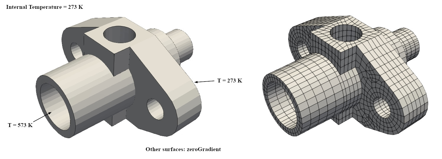Case geometry and mesh

This case computes the transient temperature distribution in a flange. It is the multiPhysicsFoam counterpart of the classic OpenFOAM laplacianFoam flange tutorial: the same geometry, mesh and boundary conditions are used, but the problem is solved through the multiPhysicsFoam framework using the laplacianFluid region type running in single-region mode.

The flange is initially at a uniform temperature of 273 K. One face is held at 273 K, while a second face is held at a hot 573 K. The remaining faces are insulated (zero heat flux). Heat then diffuses through the solid geometry over time until a steady linear distribution is approached.

The governing equation is the transient heat-conduction (diffusion) equation for a scalar temperature field $T$:

where $D_T$ is the (constant, uniform) thermal diffusivity. There is no convective transport and no source term, so the problem reduces to a pure Laplacian diffusion of $T$.

In laplacianFluid, this equation is assembled once per time step and solved implicitly for the temperature field T. Because there is only a single region and a single primitive variable, no inter-region coupling or outer PIMPLE iteration is required - the region is self-coupled on T only:

for all time-steps
    construct TEqn:  ddt(T) - laplacian(DT, T) == fvOptions(T)
    solve TEqn for T
    if writeTime():
        update derived output: grad(T), DT*grad(T)
end

At every write time, laplacianFluid also computes and writes four derived fields - the components of $\nabla T$ and the diffusive heat flux $D_T \nabla T$ - mirroring the write.H output of the original laplacianFoam solver. See Derived Output Fields below.

Case Structure

The case structure follows the typical OpenFOAM case structure:

flangeMP
├── 0
│   └── T
├── Allclean
├── Allrun
├── Allrun-parallel
├── constant
│   ├── polyMesh
│   │   └── …
│   └── transportProperties
└── system
    ├── controlDict
    ├── decomposeParDict
    ├── fvSchemes
    └── fvSolution

• 0 - initial and boundary conditions for the primitive field T.
• constant/transportProperties - the thermal diffusivity DT. Only consulted if 0/DT is not supplied.
• constant/polyMesh - the mesh (generated at run time from flange.ans).
• system - the run-time control (controlDict), discretization schemes (fvSchemes), linear-solver settings (fvSolution) and the parallel decomposition settings (decomposeParDict).

Every write time also produces four derived fields alongside T and DT: gradTx, gradTy, gradTz and DTgradT, e.g.:

3
├── DT
├── DTgradT
├── T
├── gradTx
├── gradTy
├── gradTz
└── uniform

The key entries that select the physics are in system/controlDict:

application       multiPhysicsFoam;

singleRegionMode yes;

regionType       laplacianFluid;

• application multiPhysicsFoam: the executable that is run.
• singleRegionMode yes: tells the framework there is only one region occupying the whole domain, so no constant/regionProperties/multi-region setup is required.
• regionType laplacianFluid: selects the laplacianFluid region type at runtime.

Initial Conditions and Boundary Conditions

In this case, there is a single primitive variable:

• temperature (scalar)

├── 0
│   └── T   temperature scalar field

The initial temperature field is uniform at 273 K.

Temperature Field T

The 0/T file sets the internal field and the four patch boundary conditions:

dimensions      [0 0 0 1 0 0 0];

internalField   uniform 273;

boundaryField
{
    "(patch1|patch3)"
    {
        type            zeroGradient;
    }

    patch2
    {
        type            fixedValue;
        value           uniform 273;
    }

    patch4
    {
        type            fixedValue;
        value           uniform 573;
    }
}

• patch1 and patch3 use zeroGradient, i.e. insulated walls with no heat flux ($\nabla T \cdot \boldsymbol{n} = 0$).
• patch2 is held at a fixed temperature of 273 K.
• patch4 is held at a fixed hot temperature of 573 K.

The dimensions [0 0 0 1 0 0 0] indicate that T is a temperature in kelvin.

Transport Properties

The only physical property required is the thermal diffusivity DT, specified in constant/transportProperties:

DT              4e-05;

DT has the dimensions of a diffusivity (m²/s). In the solver it is read as a dimensionedScalar with dimViscosity; if a DT field is not present in the time directory, this uniform value is used to construct one.

constant/transportProperties is only consulted when 0/DT is absent, exactly as in laplacianFoam. If this case’s 0/ directory supplied a DT field directly, transportProperties would not need to exist at all. The solver checks for 0/DT first and only falls back to reading transportProperties if that check fails.

Write Control - the writeGradT switch

system/fvSolution carries one region-specific control, read from the SIMPLE subdict:

SIMPLE
{
    writeGradT      true;
}

• writeGradT true (the default, used in this case): at every write time, laplacianFluid recomputes and writes gradTx, gradTy, gradTz and DTgradT alongside T - reproducing laplacianFoam’s write.H output exactly.
• writeGradT false: only T (and DT) are written. No gradTx/gradTy/gradTz/DTgradT field objects are even constructed, which is useful in coupled multi-region cases where these four extra fields per write are unwanted overhead.

If the SIMPLE subdict or the writeGradT entry is absent entirely, the default (true) applies.

Running the Case

As in all multiPhysicsFoam tutorials, the case is run using the included Allrun script, i.e. > ./Allrun. In this case, the Allrun script is:

#!/bin/sh
cd "${0%/*}" || exit                                # Run from this directory
. ${WM_PROJECT_DIR:?}/bin/tools/RunFunctions        # Tutorial run functions
#------------------------------------------------------------------------------

restore0Dir

runApplication ansysToFoam \
    ${FOAM_TUTORIALS:?}/resources/geometry/flange.ans -scale 0.001

runApplication $(getApplication)

if true
then
    runApplication foamToEnsight -noZero
    runApplication foamToVTK
fi

#------------------------------------------------------------------------------

The script first restores the initial 0 directory, then converts the ANSYS mesh (flange.ans) supplied with the OpenFOAM tutorials into the OpenFOAM format using ansysToFoam (with a scale factor of 0.001 to convert mm to m). The $(getApplication) call reads the application entry from system/controlDict (here multiPhysicsFoam) and runs it. Finally the results are converted to EnSight and VTK formats for post-processing.

Examining the Solver Output

Let us examine the output from the multiPhysicsFoam solver for this case. At start-up, the framework reports the region it has created and the coupling mode:

Creating multi-region system

Creating regions:
Creating region region0: laplacianFluid
Selecting regionType: laplacianFluid

SIMPLE: no convergence criteria found. Calculations will run for 3 steps.

No PIMPLE active

Creating region interfaces:

Since this is a single-region case, no region interfaces are created. Each time step then reports the assembly and solution of the temperature equation:

Time = 0.005
Time step = 0.005 Index = 1

Solved region specific physics in 0 s.
Constructing TEqn of laplacianFluid

Solving for T in laplacianFluid
DICPCG:  Solving for T, Initial residual = 1, Final residual = 1.65094e-07, No Iterations 5
Solved self-coupled region equations in 0 s.
ExecutionTime = 0.05 s  ClockTime = 0 s

The important lines are:

• Constructing TEqn of laplacianFluid: the region type assembles its temperature matrix TEqn for this time step.
• Solving for T in laplacianFluid: the equation is handed to the linear solver.
• DICPCG: Solving for T, Initial residual = …, Final residual = …, No Iterations …: the linear-solver report from the DIC-preconditioned conjugate gradient (PCG) solver selected in fvSolution.
• Solved self-coupled region equations in … s.: confirms that the region has been solved on its self-coupled field (T), with no partitioned inter-region coupling involved.

As the simulation progresses, the initial residual for T steadily decreases from 1 towards small values, indicating the temperature field is converging towards its final distribution as heat diffuses through the flange:

Time = 0.01
DICPCG:  Solving for T, Initial residual = 0.20412, Final residual = 3.82655e-07, No Iterations 4

Time = 0.015
DICPCG:  Solving for T, Initial residual = 0.110105, Final residual = 2.15393e-07, No Iterations 4

Time = 0.02
DICPCG:  Solving for T, Initial residual = 0.0728725, Final residual = 1.58276e-07, No Iterations 4

Results (validation):

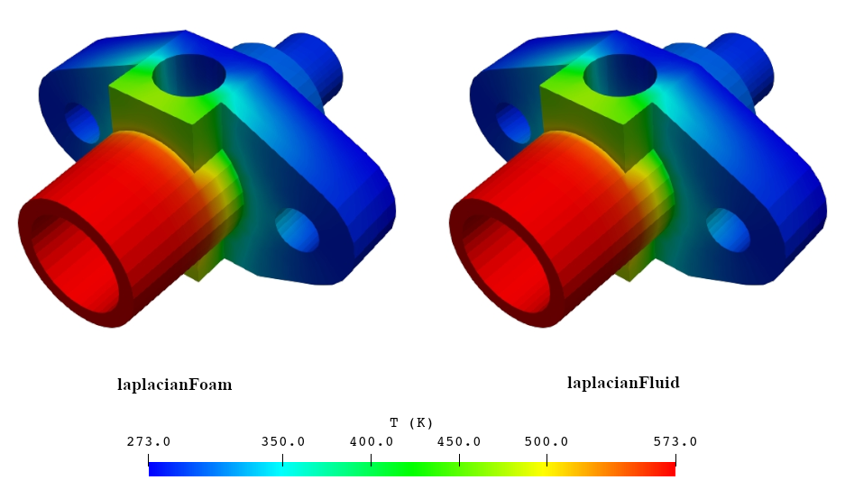
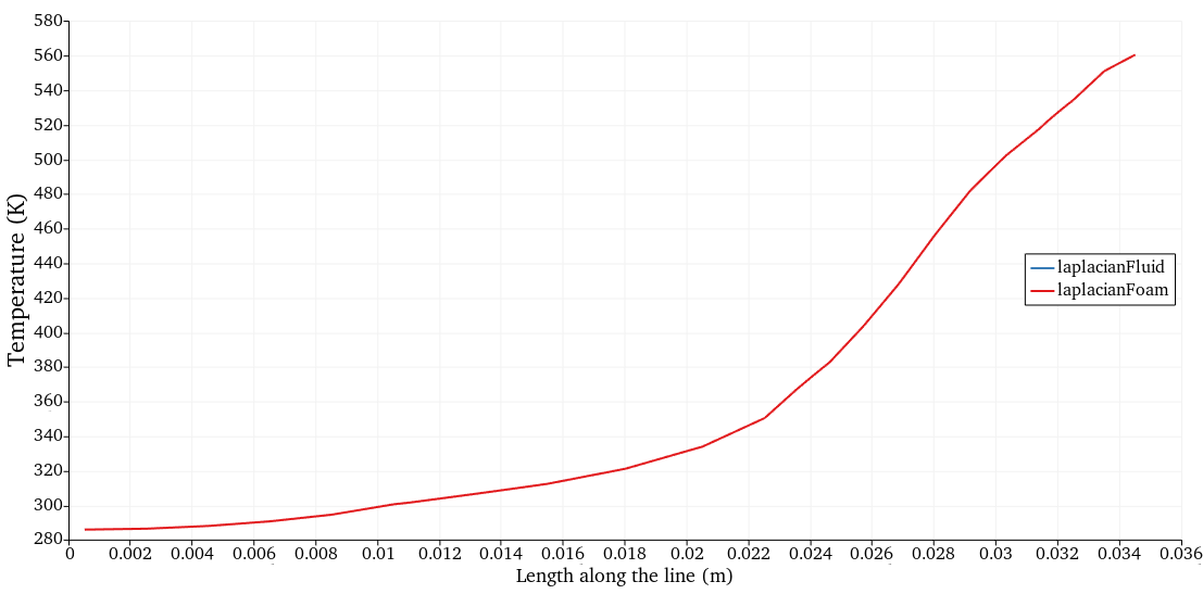
Following are the Temperature contour plots and line plots for this case, solved using laplacianFoam and laplacianFluid. As it can be observed, both solutions match, hence validating the correct porting of laplacianFoam to laplacianFluid.