Shell and Tube Heat Exchanger
Repository path: tutorials/conjugateHeatTransfer/ShellAndTubeHeatExchanger
Reference: Alkafri et al. (2024), multiRegionFoam: A Unified Multiphysics Framework, Sect. 7.2
Overview
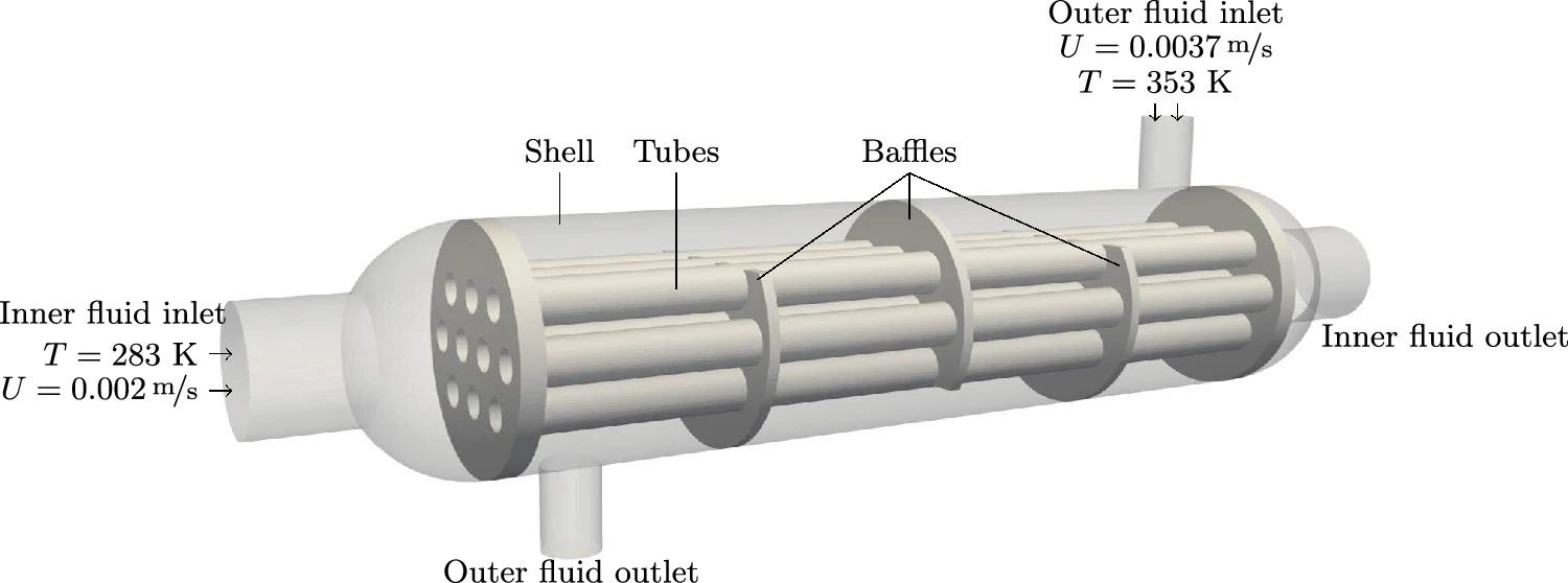
Fig. 10 — Geometry of the shell-and-tube heat exchanger with inner fluid inlet (T=283 K, U=0.002 m/s) and outer fluid inlet (T=353 K, U=0.0037 m/s).
This case demonstrates an industrial conjugate heat transfer application: a shell-and-tube heat exchanger with a shell, tubes, and baffles. Heat transfer occurs between two fluids:
- Inner fluid — flows at lower temperature inside the tubes ($T = 283\,\text{K}$, $U = 0.002\,\text{m/s}$)
- Outer fluid — flows within the shell but outside the tubes ($T = 353\,\text{K}$, $U = 0.0037\,\text{m/s}$)
Solid tube walls prevent mixing; baffles direct the shell-side flow. The case setup is based on a publicly available SimScale GmbH reference case.
The simulations are run for 500 s with a time step $\Delta t = 1\,\text{s}$. The coupled thermal boundary conditions are the same as in the flat-plate case (Table 3 in the paper).
Boundary conditions
Table: Boundary conditions for the heat exchanger
| Boundary | Thermal | Velocity |
|---|---|---|
| Inner fluid | ||
| inlet | 283 K | (0.002 0 0)ᵀ m/s |
| inner_to_solid | coupled | (0 0 0)ᵀ m/s |
| outlet, walls | zeroGradient | zeroGradient |
| Outer fluid | ||
| inlet | 353 K | (0 0.0037 0)ᵀ m/s |
| outer_to_solid | coupled | (0 0 0)ᵀ m/s |
| outlet, walls | zeroGradient | zeroGradient |
| Solid | ||
| solid_to_inner | coupled | – |
| solid_to_outer | coupled | – |
| walls | zeroGradient | – |
Material properties
Table: Thermophysical properties of fluid and solid
| Property | Symbol | Unit | Fluid | Solid |
|---|---|---|---|---|
| Density | ρ | kg/m³ | 1027 | 8960 |
| Thermal conductivity | k | W/m·K | 0.668 | 401 |
| Dynamic viscosity | μ | kg/ms | 3.645 × 10⁻⁴ | – |
| Specific heat capacity | c_p | J/kg·K | 4195 | 385 |
Both inner and outer fluids share the same material properties.
Numerical schemes
Table: Numerical schemes
| Scheme | Setting |
|---|---|
ddtScheme | steadyState |
gradScheme | Gauss linear |
gradScheme grad(U) | cellLimited Gauss linear 1 |
divScheme div(phi,U) | Gauss upwind |
divScheme div(phi,T) | Gauss upwind |
laplacianScheme | Gauss linear corrected |
interpolationScheme | linear |
snGradScheme | corrected |
Mesh
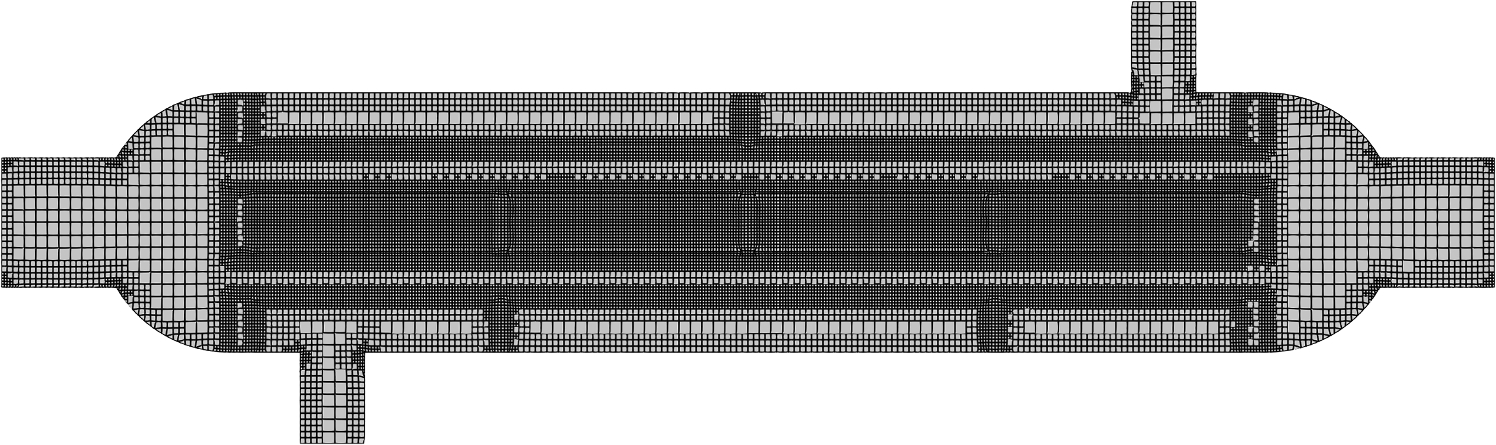
Fig. 11 — Computational mesh for the shell-and-tube heat exchanger simulation.
Results summary
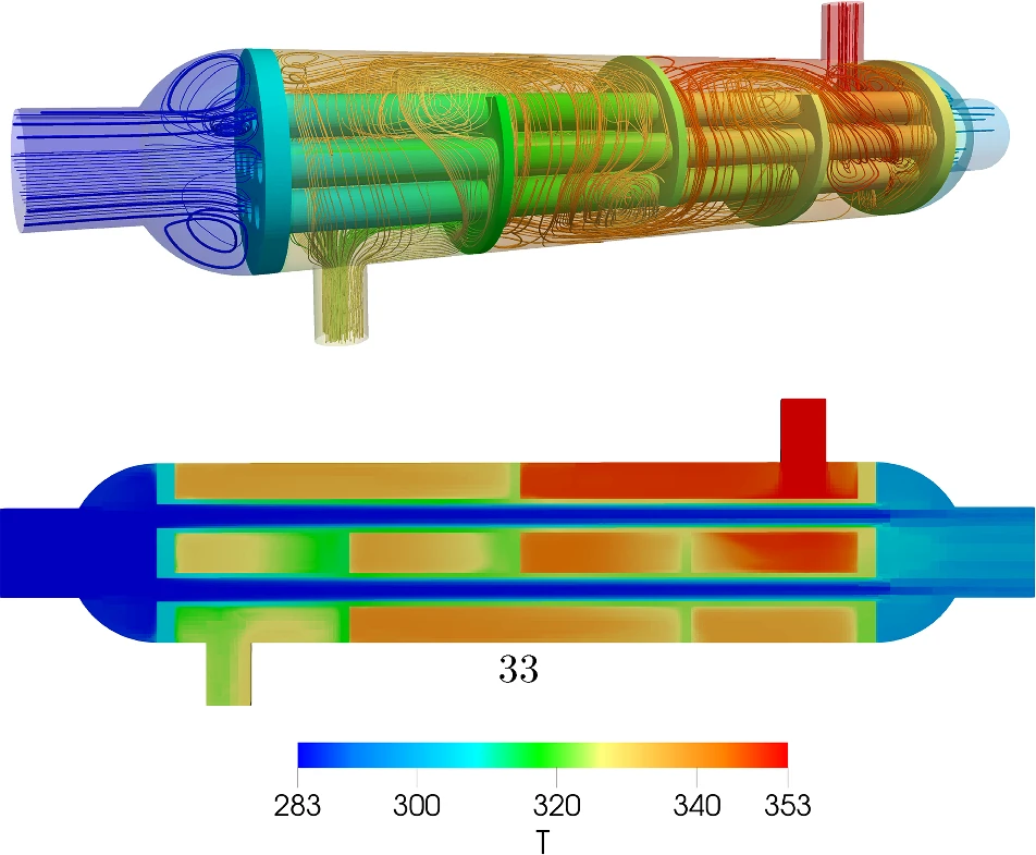
Fig. 12 — Final temperature distribution at t = 30 s using monolithic coupling (temperature range 283–353 K).
The final temperature distribution (t = 30 s) shows no significant change thereafter, confirming a steady state is reached around t = 500 s. Both partitioned (Aitken relaxation) and monolithic coupling produce comparable field values; the partitioned approach takes longer to reach steady state.
Running the case
cd $FOAM_RUN/../multiPhysicsFoam/tutorials/conjugateHeatTransfer/ShellAndTubeHeatExchanger
./Allrun