Flow Over Heated Plate
Repository path: tutorials/conjugateHeatTransfer/flowOverHeatedPlate
Reference: Alkafri et al. (2024), multiRegionFoam: A Unified Multiphysics Framework, Sect. 7.1
Overview
An incompressible laminar flow over a flat plate of finite thickness is considered. A fluid of uniform temperature $T_\infty = 300\,\text{K}$ and velocity $U_\infty = 1\,\text{m/s}$ flows over a plate of length $L = 1\,\text{m}$ held at a constant bottom temperature $T_s = 310\,\text{K}$.
The aspect ratio is fixed at $\lambda = a/L = 0.25$. Results are validated against the numerical and analytical reference solutions from Vynnycky et al., computing the dimensionless conjugate boundary temperature
$$\theta = \frac{T - T_\infty}{T_s - T_\infty}.$$Computational domain
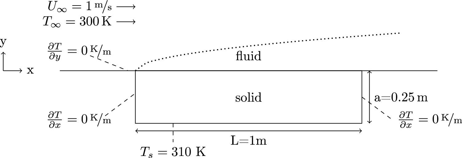
Fig. 7 — Computational domain and boundary conditions for the flow over a heated plate.
Boundary conditions
Table: General boundary conditions
| Boundary | Thermal | Velocity |
|---|---|---|
| Fluid | ||
| inlet | 300 K | (1 0 0)ᵀ m/s |
| bottom (no-slip, plate) | coupled | (0 0 0)ᵀ m/s |
| slip-bottom (before plate) | zeroGradient | zeroGradient |
| outlet, top | zeroGradient | zeroGradient |
| Solid | ||
| top | coupled | – |
| bottom | 310 K | – |
| left, right | zeroGradient | – |
Table: Coupled thermal boundary conditions at the fluid–solid interface
| Region | Boundary | Partitioned | Monolithic |
|---|---|---|---|
| Fluid | bottom | regionCoupledTemperatureJump | monolithicTemperature |
| Solid | top | regionCoupledHeatFlux | monolithicTemperature |
Material properties
Table: Thermophysical properties of fluid and solid
| Property | Symbol | Unit | Solid | Fluid |
|---|---|---|---|---|
| Density | ρ | kg/m³ | 1 | 1 |
| Dynamic viscosity | μ | kg/ms | – | ρ_f U∞ L / Re |
| Thermal conductivity | k | W/m·K | 100 | k_s / k |
| Specific heat capacity | c_p | J/kg·K | 100 | k_f Pr / μ |
Mesh
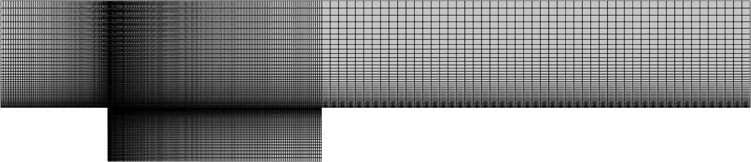
Fig. 8 — Meshes for the flow over a heated plate simulation. Both fluid and solid regions use hexahedral elements with mesh grading towards the fluid–solid interface.
Parameter study
Table: Simulated parameter combinations
| Re | Pr | k |
|---|---|---|
| 500 | 0.01 | 1, 5, 20 |
| 10 000 | 0.01 | 1, 5, 20 |
| 500 | 100 | 1, 5, 20 |
Simulations are run for 10 s with a time step $\Delta t = 0.01\,\text{s}$.
Numerical schemes
Table: Numerical schemes
| Scheme | Setting |
|---|---|
ddtScheme | backward |
gradScheme | leastSquares |
divScheme div(phi,U) | Gauss upwind |
divScheme div(phi,T) | Gauss linearUpwind Gauss linear |
laplacianScheme | Gauss linear corrected |
interpolationScheme | linear |
snGradScheme | corrected |
Results summary
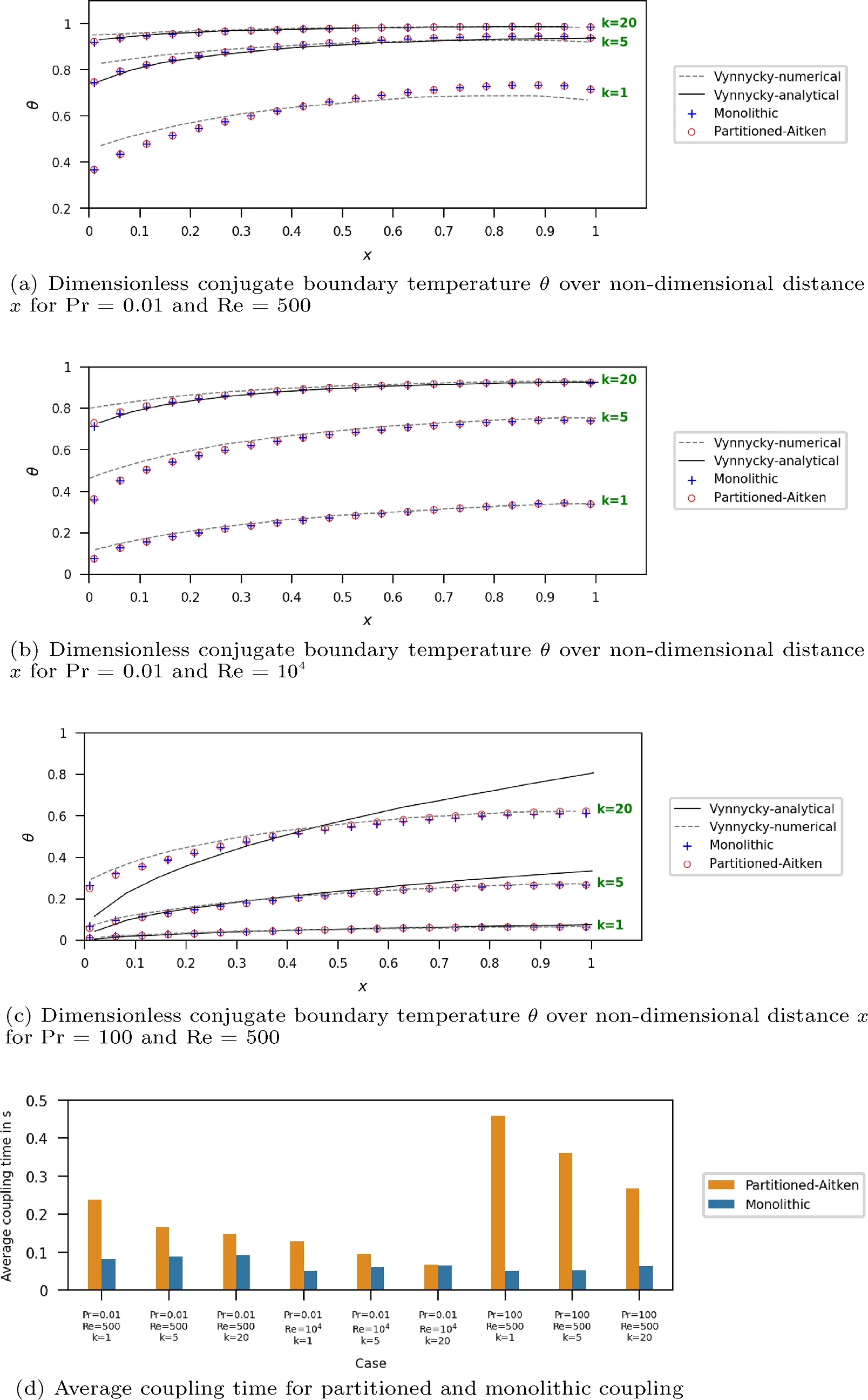
Fig. 9 — Simulation results for different Pr, Re, and k values. (a) θ for Pr=0.01, Re=500. (b) θ for Pr=0.01, Re=10⁴. (c) θ for Pr=100, Re=500. (d) Average coupling time for partitioned (Aitken) and monolithic coupling.
Both monolithic and partitioned (Aitken relaxation) coupling reproduce the reference solutions from Vynnycky et al. for all Pr, Re, and k combinations. Monolithic coupling exhibits lower or equal average coupling time compared to partitioned coupling across all cases, with the most notable advantage at Pr = 100 where monolithic coupling time is nearly constant.
Running the case
cd $FOAM_RUN/../multiPhysicsFoam/tutorials/conjugateHeatTransfer/flowOverHeatedPlate

# Partitioned coupling — serial
./Allrun --partitioned --serial

# Partitioned coupling — parallel
./Allrun --partitioned --parallel
Note
Monolithic coupling is not yet supported for this case via theAllrun script.